Q-learning
Q-Learning이라는 놈은 off-policy value-based method that use TD approach to train its action-value function이다.
중요한 점은
- off-policy
- value-based : 최적의 policy를 찾기위해서 각 state의 action pair의 value를 계산한다.
- TD approach : episode의 전체 rewoard를 계산할 수 없기 때문에 다음 state의 reward를 할인해서 value를 계산한다.
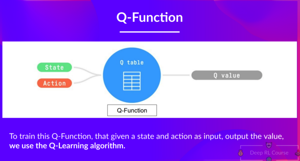
Q-learning은 Q value를 최대화하는 Q-Function을 찾는 것이다!
여기서 Q-Function은 Q-table로 표현된다.
Example
위 그림은 예제인데 쥐가 가장 큰 reward를 받기 위한 방법을 이야기한다.
최초에 Q-talbe은 0으로 초기화 되고 action과 state pair의 2차원 table을 가진다. 이때 쥐가 선택할 수 있는 action은 오른쪽으로 가거나 아래쪽으로 가는 방향이다. 이러한 관계를 통해 state-action pair를 업데이트 해나가는 것이 Q-learning의 중점이다.
결과적으로 이러한 방법을 통해 Q-function을 찾게 되고 이는 Q-table로 표현이 되는 것이다.
아래는 Q-learning의 presudo Code이다.
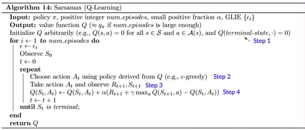
위 코드를 쥐돌이를 통해서 구현하면 아래와 같다.
# 사용할 Lib import
import numpy as np
import pandas as pd
import random as r

episode = 10000
learning_rate = 0.001
eplison = 1

# graph를 통해 쥐돌이 판 만들기
graph = np.empty((0,3))
graph = np.append(graph,np.array([[0,0,1]]),axis=0)
graph = np.append(graph,np.array([[1,-10,10]]),axis=0)

# 위아래를 움직이는 것 확인
col = ['up', 'down', 'left', 'right']
col_ = [(-1,0),(1,0),(0,-1),(0,1)]
index = [(i,j) for i in range (2) for j in range (3)]


# Q-table 생성
df = pd.DataFrame(0.000000,index=index, columns=col)

# policy를 정의하는 2개의 함수
# epslison 값에 따라서 random -> random_policy()
# 그렇지 않을 경우에는 greedy_policy()
# now => 현재 위치
def random_policy(now):
  s_next=()
  while True:
    a = r.randint(0,3)
    s_next = np.add(now,col_[a])
    if s_next[0]>-1 and s_next[0]<2 and s_next[1]>-1 and s_next[1]<3:
      return [s_next,a]

def greedy_policy(now):
  ret_next = ()
  ret_action =  -1
  s_next=()
  max_int = -int(1e9)
  for i in range(4):
    s_next = np.add(now,col_[i])
    if s_next[0]>-1 and s_next[0]<2 and s_next[1]>-1 and s_next[1]<3 and max_int < graph[s_next[0],s_next[1]]:
      ret_next = s_next
      max_int = graph[s_next[0],s_next[1]]
      ret_action =i
  return [ret_next,ret_action]

now=(0,0)

# v <- v + aplha(reward + gamma * v(st+1) - v(s))
# value_function은 몬테카를로에 의한 TD없데이트를 의미한다.
def value_function(s_now, s_next, action):
  global learning_rate
  update_value = df.at[s_now,col[action]] + learning_rate * (graph[s_next[0]][s_next[1]] + 0.99 * df.at[s_next,col[action]] - df.at[s_now,col[action]])
  df.at[s_now,col[action]] = update_value


for i in range(episode):
  ret_set = []
  if eplison >0.3:
    ret_set = random_policy(now)
  else:
    ret_set = greedy_policy(now)
  value_function(now, (ret_set[0][0],ret_set[0][1]), ret_set[1])
  now = (ret_set[0][0],ret_set[0][1])
  eplison -=0.0001
  print(df)
  print(eplison)


df = df.replace(1,0)
print(df)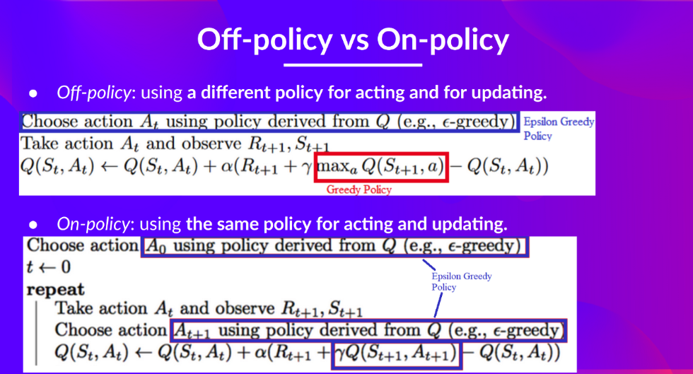
Off-policy와 On-policy는 위의 설명 처럼
- Off-policy : 액션을 선택하는 함수와 업데이트하는 함수가 다르다.
- On-policy : 액선을 선택하는 함수와 업데이트 하는 함수가 같다.
다음에는 Unit3 - DQN에대해서 공부한다.